In this tutorial, we will introduce and explain Smith Charts, and then given an introduction
to impedance matching. We will then
use the Smith Chart to perform impedance matching with
transmission lines
and lumped components (capacitors and inductors).
The Smith Chart is a fantastic tool for visualizing the
impedance
of a transmission line and antenna system as a function of frequency.
Smith Charts can be used to increase understanding of
transmission lines
and how they behave from an impedance viewpoint. Smith Charts are also
extremely helpful for impedance matching, as we will see. The Smith Chart is
used to display an actual (physical) antenna's impedance when measured on a Vector Network Analyzer (VNA).
Smith Charts were originally developed around 1940 by Phillip Smith as a useful tool for making
the equations
involved in transmission lines easier to manipulate. See, for instance,
the input impedance
equation for a load attached to a transmission line of length L and characteristic impedance
Z0. With modern computers, the Smith Chart is no longer used to the simplify the calculation of
transmission line equatons; however, their value in visualizing the impedance of an antenna or
a transmission line has not decreased.
The Smith Chart is shown in Figure 1. A larger version is shown
here.
Figure 1. The basic Smith Chart.
Figure 1 should look a little intimidating, as it appears to be lines going everywhere.
There is nothing to fear though. We will build up the Smith Chart from scratch, so that
you can understand exactly what all of the lines mean. In fact, we are going to learn
an even more complicated version of the Smith Chart known as the
immitance Smith Chart, which is twice as complicated, but also twice as useful. But
for now, just admire the Smith Chart and its curvy elegance.
This section of the antenna theory site will present an introduction to Smith Chart basics.
Smith Chart Tutorial
We'll now begin to explain the fundamentals of the Smith Chart. The Smith Chart displays the complex reflection coefficient [Equation 1, below],
in polar form, for an arbitrary impedance (we'll call the impedance ZL or the load impedance). The reflection coefficient is completely determined
by the impedance ZL and the "reference" impedance Z0. Note that Z0 can be viewed as the impedance of the transmitter, or
what is trying to deliver power to the antenna. Hence, the Smith Chart is a graphical method of displaying the impedance of an antenna, which
can be a single point or a range of points to display the impedance as a function of frequency.
For a primer on complex math, click here.
Recall that the complex reflection coefficient ()
for an impedance ZL attached to a transmission line with
characteristic impedance
Z0 is given by:
[Equation 1]
For this Smith Chart tutorial, we will assume Z0 is 50 Ohms, which is often, but not always the case.
Note that the Smith Chart can be used with any value of Z0.
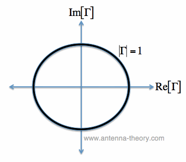
The complex reflection coefficient, or , must have a magnitude between
0 and 1.
As such, the set of all possible values for must lie within
the unit circle:
Figure 2. The Complex Reflection Coefficient must lie somewhere within the unit circle.
In Figure 2, we are plotting the set of all values for the complex reflection coefficient, along the
real and imaginary axis. The center of the Smith Chart is the point where the reflection coefficient
is zero. That is, this is the only point on the Smith Chart where no power is reflected by the
load impedance.
The outter ring of the Smith Chart is where the magnitude of
is equal to 1. This is the black circle in Figure 1.
Along this curve, all of the power is reflected by the load impedance.
Let's look at a few examples.
Smith Chart Example 1. Suppose =0.5.
From equation [1], we can solve for ZL to be:
[Equation 2]
From equation [2], with Z0=50 Ohms, a reflection coefficient of 0.5 corresponds to a load impedance ZL=150 Ohms.
We can plot gamma_1 on the smith chart:
.
Figure 3. plotted on the Smith Chart.
Since is entirely real, the point lies along the real gamma axis (x-axis) in Figure 3,
and the imaginary axis value (y-axis) location is 0.
Smith Chart Example 2. Suppose = -0.3 + i0.4
is plotted on the Smith Chart in Figure 4:
Figure 4. plotted on the Smith Chart.
From Equation [2] and using Z0=50, we note that corresponds to a load impedance
ZL = 20.27 + i*21.62 [Ohms].
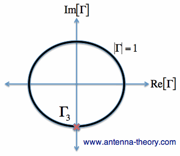
Smith Chart Example 3. = -i.
is plotted on the Smith Chart in Figure 5:
Figure 5. =-i plotted on the Smith Chart.
From Equation [2] and with Z0=50, corresponds to a load impedance ZL = -i*50 Ohms. That is,
the load impedance here is purely imaginary and negative, which indicates a purely capacitive load.
VSWR on the Smith Chart
Since VSWR
is only a function of the absolute value of , we can get the VSWR for a load from the Smith Chart as well.
That is, a VSWR = 1 would be the center of the Smith Chart, and VSWR=3 would be a circle centered around the center of the Smith
Chart, with magnitude =0.5. Circles centered at the origin of the Smith Chart are constant-VSWR circles.
Note that the outer boundary of the Smith Chart (where =1) corresponds to a VSWR of infinity.
 =0.5.
=0.5.  .
.
 )
for an impedance ZL attached to a transmission line with
)
for an impedance ZL attached to a transmission line with
 is equal to 1. This is the black circle in Figure 1.
Along this curve, all of the power is reflected by the load impedance.
is equal to 1. This is the black circle in Figure 1.
Along this curve, all of the power is reflected by the load impedance. 
 = -0.3 + i0.4
 plotted on the Smith Chart.
 = -i.
= -i. corresponds to a load impedance ZL = -i*50 Ohms. That is,
the load impedance here is purely imaginary and negative, which indicates a purely capacitive load.
corresponds to a load impedance ZL = -i*50 Ohms. That is,
the load impedance here is purely imaginary and negative, which indicates a purely capacitive load.